Small-angle approximation

Approximately equal behavior of some (trigonometric) functions for x → 0

The small-angle approximations can be used to approximate the values of the main trigonometric functions, provided that the angle in question is small and is measured in radians:

${\begin{aligned}\sin \theta &\approx \theta \\\cos \theta &\approx 1-{\frac {\theta ^{2}}{2}}\approx 1\\\tan \theta &\approx \theta \end{aligned}}$

These approximations have a wide range of uses in branches of physics and engineering, including mechanics, electromagnetism, optics, cartography, astronomy, and computer science. One reason for this is that they can greatly simplify differential equations that do not need to be answered with absolute precision.

There are a number of ways to demonstrate the validity of the small-angle approximations. The most direct method is to truncate the Maclaurin series for each of the trigonometric functions. Depending on the order of the approximation, $\textstyle \cos \theta$ is approximated as either $1$ or as ${\textstyle 1-{\frac {\theta ^{2}}{2}}}$.

Justifications

Graphic

The accuracy of the approximations can be seen below in Figure 1 and Figure 2. As the measure of the angle approaches zero, the difference between the approximation and the original function also approaches 0.

• 
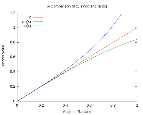  Figure 1. A comparison of the basic odd trigonometric functions to θ. It is seen that as the angle approaches 0 the approximations become better.
• 
  Figure 2. A comparison of cos θ to 1 − θ²/2. It is seen that as the angle approaches 0 the approximation becomes better.

Geometric

The red section on the right, d, is the difference between the lengths of the hypotenuse, H, and the adjacent side, A. As is shown, H and A are almost the same length, meaning cos θ is close to 1 and θ²/2 helps trim the red away.

$$\cos {\theta }\approx 1-{\frac {\theta ^{2}}{2}}$$

The opposite leg, O, is approximately equal to the length of the blue arc, s. Gathering facts from geometry, s = Aθ, from trigonometry, sin θ = O/H and tan θ = O/A, and from the picture, O ≈ s and H ≈ A leads to:

$$\sin \theta ={\frac {O}{H}}\approx {\frac {O}{A}}=\tan \theta ={\frac {O}{A}}\approx {\frac {s}{A}}={\frac {A\theta }{A}}=\theta .$$

Simplifying leaves,

$$\sin \theta \approx \tan \theta \approx \theta .$$

Calculus

Using the squeeze theorem, we can prove that

$$\lim _{\theta \to 0}{\frac {\sin(\theta )}{\theta }}=1,$$

which is a formal restatement of the approximation $\sin(\theta )\approx \theta$ for small values of θ.

A more careful application of the squeeze theorem proves that

$$\lim _{\theta \to 0}{\frac {\tan(\theta )}{\theta }}=1,$$

from which we conclude that $\tan(\theta )\approx \theta$ for small values of θ.

Finally, L'Hôpital's rule tells us that

$$\lim _{\theta \to 0}{\frac {\cos(\theta )-1}{\theta ^{2}}}=\lim _{\theta \to 0}{\frac {-\sin(\theta )}{2\theta }}=-{\frac {1}{2}},$$

which rearranges to ${\textstyle \cos(\theta )\approx 1-{\frac {\theta ^{2}}{2}}}$ for small values of θ. Alternatively, we can use the double angle formula $\cos 2A\equiv 1-2\sin ^{2}A$. By letting $\theta =2A$, we get that ${\textstyle \cos \theta =1-2\sin ^{2}{\frac {\theta }{2}}\approx 1-{\frac {\theta ^{2}}{2}}}$.

Algebraic

The small-angle approximation for the sine function.

The Maclaurin expansion (the Taylor expansion about 0) of the relevant trigonometric function is

$${\begin{aligned}\sin \theta &=\sum _{n=0}^{\infty }{\frac {(-1)^{n}}{(2n+1)!}}\theta ^{2n+1}\\&=\theta -{\frac {\theta ^{3}}{3!}}+{\frac {\theta ^{5}}{5!}}-{\frac {\theta ^{7}}{7!}}+\cdots \end{aligned}}$$

where θ is the angle in radians. In clearer terms,

$$\sin \theta =\theta -{\frac {\theta ^{3}}{6}}+{\frac {\theta ^{5}}{120}}-{\frac {\theta ^{7}}{5040}}+\cdots$$

It is readily seen that the second most significant (third-order) term falls off as the cube of the first term; thus, even for a not-so-small argument such as 0.01, the value of the second most significant term is on the order of 0.000001, or 1/10000 the first term. One can thus safely approximate:

$$\sin \theta \approx \theta$$

By extension, since the cosine of a small angle is very nearly 1, and the tangent is given by the sine divided by the cosine,

$$\tan \theta \approx \sin \theta \approx \theta ,$$

Dual numbers

One may use dual numbers, denoted ε, often considered similar to an infinitesimal amount, with a square of 0. By using the Maclaurin series of cosine and sine and substituting θ=θε, the result is cos(θε)=1 and sin(θε)=θε. These approximations satisfy the Pythagorean identity:

cos²(θε)+sin²(θε)=1²+(θε)²=1+θ²ε²=1+θ²0=1.

Error of the approximations

Figure 3. A graph of the relative errors for the small angle approximations.

Figure 3 shows the relative errors of the small angle approximations. The angles at which the relative error exceeds 1% are as follows:

• cos θ ≈ 1 at about 0.1408 radians (8.07°)
• tan θ ≈ θ at about 0.1730 radians (9.91°)
• sin θ ≈ θ at about 0.2441 radians (13.99°)
• cos θ ≈ 1 − θ²/2 at about 0.6620 radians (37.93°)

Angle sum and difference

The angle addition and subtraction theorems reduce to the following when one of the angles is small (β ≈ 0):

cos(α + β)	≈ cos(α) − β sin(α),
cos(α − β)	≈ cos(α) + β sin(α),
sin(α + β)	≈ sin(α) + β cos(α),
sin(α − β)	≈ sin(α) − β cos(α).

Specific uses

Astronomy

In astronomy, the angular size or angle subtended by the image of a distant object is often only a few arcseconds (denoted by the symbol ″), so it is well suited to the small angle approximation. The linear size (D) is related to the angular size (X) and the distance from the observer (d) by the simple formula:

$D=X{\frac {d}{206\,265{''}}}$

where X is measured in arcseconds.

The quantity 206265″ is approximately equal to the number of arcseconds in a circle (1296000″), divided by 2π, or, the number of arcseconds in 1 radian.

The exact formula is

$D=d\tan \left(X{\frac {2\pi }{1\,296\,000{''}}}\right)$

and the above approximation follows when tan X is replaced by X.

Motion of a pendulum

The second-order cosine approximation is especially useful in calculating the potential energy of a pendulum, which can then be applied with a Lagrangian to find the indirect (energy) equation of motion.

When calculating the period of a simple pendulum, the small-angle approximation for sine is used to allow the resulting differential equation to be solved easily by comparison with the differential equation describing simple harmonic motion.

Optics

In optics, the small-angle approximations form the basis of the paraxial approximation.

Wave Interference

The sine and tangent small-angle approximations are used in relation to the double-slit experiment or a diffraction grating to develop simplified equations like the following, where y is the distance of a fringe from the center of maximum light intensity, m is the order of the fringe, D is the distance between the slits and projection screen, and d is the distance between the slits:

$$y\approx {\frac {m\lambda D}{d}}$$

Structural mechanics

The small-angle approximation also appears in structural mechanics, especially in stability and bifurcation analyses (mainly of axially-loaded columns ready to undergo buckling). This leads to significant simplifications, though at a cost in accuracy and insight into the true behavior.

Piloting

The 1 in 60 rule used in air navigation has its basis in the small-angle approximation, plus the fact that one radian is approximately 60 degrees.

Interpolation

The formulas for addition and subtraction involving a small angle may be used for interpolating between trigonometric table values:

Example: sin(0.755)

$${\begin{aligned}\sin(0.755)&=\sin(0.75+0.005)\\&\approx \sin(0.75)+(0.005)\cos(0.75)\\&\approx (0.6816)+(0.005)(0.7317)\\&\approx 0.6853.\end{aligned}}$$

where the values for sin(0.75) and cos(0.75) are obtained from trigonometric table.

See also

• Skinny triangle
• Small oscillations of a pendulum
• Versine and haversine
• Exsecant and excosecant